Neural Networks

I believe it makes most sense for me to start my first-ever blog with Neural Networks, as this is where I want to specialize.

Before going into technical details and all the mathematics behind of Neural Networks, I want to talk a bit about what it actually is. It’s a cheap shot to “copy” human brain, using a unit called artificial neurons to process data and recognize patterns. And for our “Hello, World!” I will be talking about MNIST dataset neural network, a machine learning model trained to recognize handwritten digits ranging from 0 to 9. It’s important to keep in mind that this is a Feedforward Neural Network (FNN).

This system has four key parts. First is the input layer, where the model takes in raw data, such as pixels of a handwritten digit (or words from text, though not for MNIST). Second are the hidden layers, which sit between the input and output where the computer does the math to find patterns. Third is the output layer, which, as name suggests, gives the final answer/prediction. Fourth are the weights and biases. And yeah, it would be really fun and easy if this was how things simply played out, but (un)fortunately, this is a really high-level overview of what’s actually happening. So let me go a bit more into detail.

It is also important to understand what values neurons hold. Normalized MNIST inputs are between 0 and 1, but a neuron’s value depends on its activation function. For example, ReLU outputs can be any non-negative number, while the output probabilities produced by softmax are between 0 and 1.

• Input Layer: A $28 \times 28$ pixel image is flattened into a one-dimensional vector of 784 values. Each hidden neuron receives all 784 input values through separate weighted connections. For hidden neuron $j$, the weighted sum before activation is

$$z_j = \sum_{i=1}^{784} w_{ji}x_i + b_j,$$

where $x_i$ is input pixel $i$, $w_{ji}$ is the weight connecting input $i$ to neuron $j$, and $b_j$ is that neuron’s bias.

• Hidden Layer: The raw value $z_j$ is passed through a non-linear activation function such as ReLU:

$$a_j = \operatorname{ReLU}(z_j) = \max(0, z_j).$$

Here, $a_j$ is the neuron’s activation. Without non-linear activation functions, multiple layers would collapse into a single transformation and the network could only model linear decision boundaries. This process repeats through every hidden layer in the network and becomes more expressive as the network gets deeper.

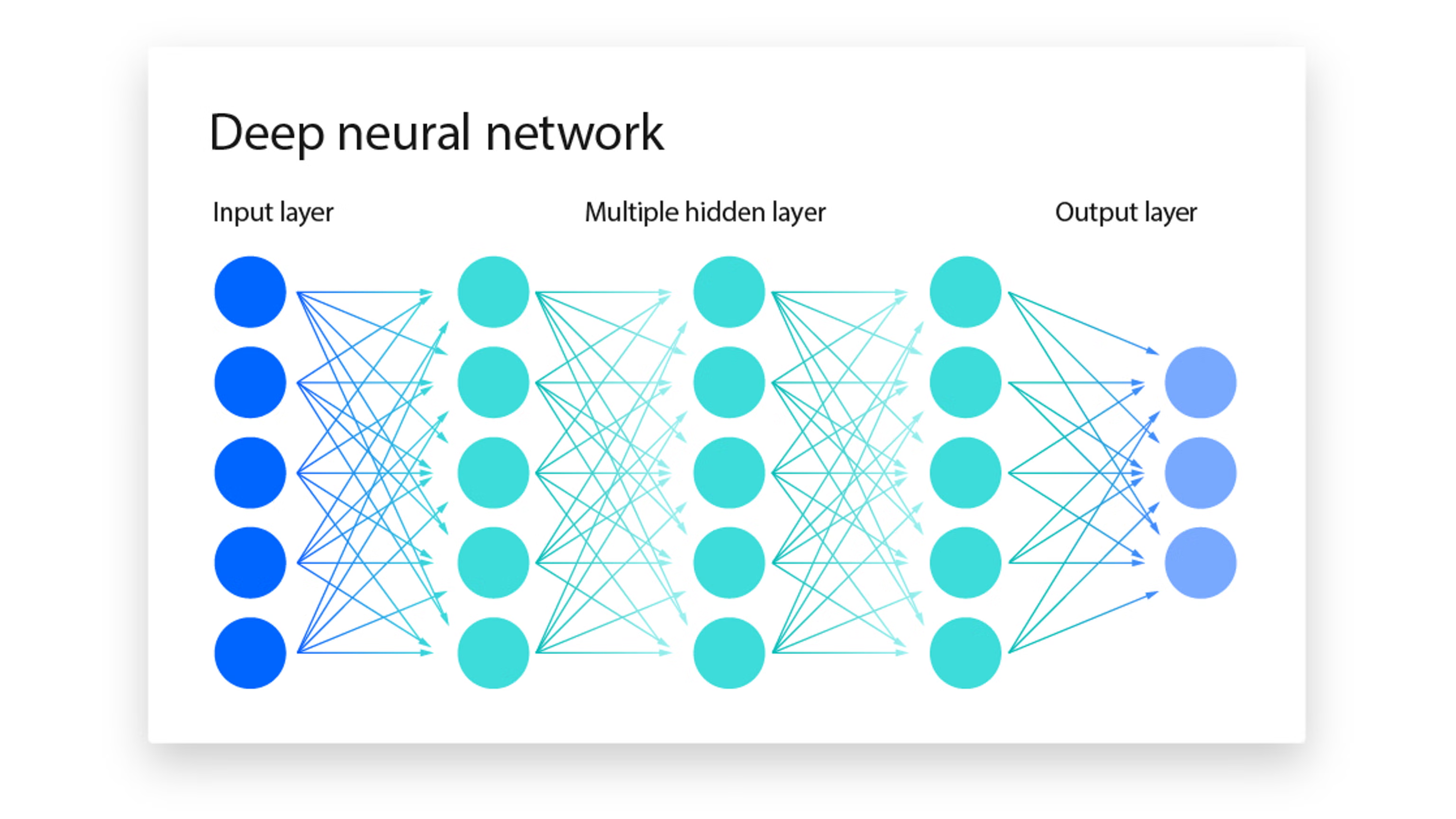
Image source: IBM, “What Is a Neural Network?”.

• Output Layer: The final hidden layer connects to an output layer consisting of 10 nodes, one for each digit from 0 to 9. Its raw outputs are called logits. To distinguish them from the hidden neuron’s value $z_j$, let $o_i$ represent output logit $i$. Softmax converts each output logit into a normalized probability $\hat{y}_i$:

$$\hat{y}_i = \operatorname{softmax}(\mathbf{o})_i = \frac{e^{o_i}}{\sum_{k=0}^{9} e^{o_k}}.$$

The probabilities are each between 0 and 1 and sum to 1. The class with the highest probability becomes the model’s prediction (i.e., the model assigns a 95% probability to digit 2):

$$\hat{c} = \operatorname*{arg\,max}_{i \in \{0, \ldots, 9\}} \hat{y}_i.$$

During training, a loss function compares this distribution with the ground-truth label. For MNIST, a common choice is cross-entropy loss:

$$\mathcal{L}(\mathbf{y}, \hat{\mathbf{y}}) = -\sum_{i=0}^{9} y_i \log(\hat{y}_i).$$

Here, $y_i$ is component $i$ of the true one-hot label vector (1 for the correct digit and 0 for every other digit), and $\hat{y}_i$ is the predicted probability. If $t$ is the true class, the sum simplifies to

$$\mathcal{L} = -\log(\hat{y}_t).$$

Backpropagation uses the chain rule to determine how much each weight and bias contributed to the loss. Gradient descent then updates all the model’s parameters, represented by $\theta$, in the direction that reduces the loss. The update from iteration $n$ to iteration $n+1$ is

$$\theta_{n+1} = \theta_n - \eta \nabla_{\theta}\mathcal{L}(\theta_n),$$

where $\theta_n$ contains the current parameter values, $\theta_{n+1}$ contains the updated values, $\mathcal{L}(\theta_n)$ is the loss produced by the current parameters, and $\eta$ is the learning rate. The term $\eta \nabla_{\theta}\mathcal{L}(\theta_n)$ is subtracted from $\theta_n$ because the gradient points in the direction in which the loss increases most quickly. Subtracting it moves the parameters in the opposite direction, toward lower loss and, hopefully, a local minimum.

In practice, training begins with randomized weight initialization, while biases are often initialized to zero. Rather than using the entire dataset for every update, training usually processes one mini-batch at a time. For each mini-batch, the network performs a forward pass, calculates the loss, and uses backpropagation to calculate the gradient of the loss with respect to every parameter. The optimizer then applies the update above. Once the model has processed every mini-batch in the training set, it has completed one epoch.

This process usually repeats for a fixed number of epochs, or early stopping ends training when performance on a validation set no longer improves. Convergence does not necessarily mean the parameters stop moving or the model reaches the minimum possible error. Neural-network loss surfaces are non-convex, so training may instead reach a useful solution where further improvements are small. The learning rate is where things can go wrong: if it is too large, training can become unstable and simply “miss” the local minimum; if it is too small, training can take too long and waste resources.